LBM

In this project we sought out to implement from scratch the Lattice Boltzmann Method for simulating fluids. Our final goal was to simulate Von Karman vortex streets, which are the series of vortices generated by a fluid flowing around an obstacle, and to compare our results with real observations.

The Method

The Lattice Boltzmann Method is a method that can be used for simulating fluids. As opposed to other methods, it doesn’t solve the Navier Stokes equations directly, but uses the Boltzmann equation to follow the statistical behaviour of the fluid. In this way, it doesn’t follow the positions and momentums of particles but rather their probability distributions.

To implement this method, one needs to define a grid over which the fluid will be described by a discrete-velocity function, from which one can calculate the density and velocity values. The method is a lot more complex than this but I won’t go into the details. See references for further information.

Implementation

We implemented a D2Q9 model (so a 2D lattice with 9 discrete velocities) with a BGK relaxation method, over a grid of 250 by 80 nodes. We set periodic conditions in the top and bottom walls, and inlet and outlet conditions in the other 2. For the obstacle, we used fullway bounce-back conditions which amount to reflecting the discrete velocities of the nodes which belong to the obstacle. We ran simulations for 15k time steps, and stored velocity, density, and vorticity information every 50 steps. We used C++ for the simulation.

Analysis

We were able to generate Von Karman vortex streets using different obstacles and Reynolds numbers. One such simulation is shown at the start of this page. We also did a set of analysis of the simulation results we got.

Size of obstacle

We changed the diameter of circular obstacles to see the effect it had on the vortices. We ran 3 simulations with increasing diameter of the obstacles. We saw that as the obstacle became larger, the size of the vortices, as well as the vortex shedding frequency, increases. We obtained this frequency by doing a fourier analysis of the vorticity data. Our results make sense given the effect that keeping the Reynolds number the same has on the systems, which amounts to simply a change of scale.

Shape of obstacle

We compared the vortices generated by a circular and a rectangular obstacle with the same characteristic length. We found that the vortices started shedding sooner with the cricle, and that the shedding frequency was higher with the rectangle.

Strouhal number and comparison with experimental data

Lastly, we ran 12 simulations with varying Reynolds numbers, and saw the relation of these numbers with the Strouhal number - which is another adimensional parameter that describes a system, it is defined as: $St = \frac{fL}{U}$ , with $f$ the vortex shedding freq., $L$ the characteristic length, and $U$ the initial velocity of the fluid. The relation between $Re$ and $St$ has been studied previously with real experiments and it has the form: $St = St^* + m/\sqrt{Re}$. In the next figure we have the points obtained from our simulation as well as the lines oobtained by experimental works. We found a good agreement, with errors associated to the parameters $St^*$ and $m$ of 0.8% and 6%, respectively. This result further confirms that the simulation works well. It’s worth noting that we’d get a better agreement with the expected behaviour by increasing the frequency of data saving (which was set to 50 timesteps).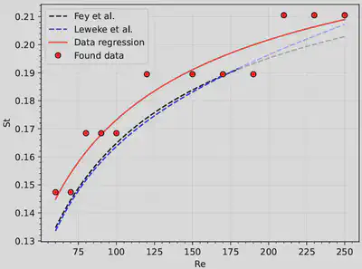

Resources

• Final report
• Final presentation
• Code repository

Acknowledgments

This project was done by me and Lizeth González