Automated Heat Capacity Measurement
 Preview of the automated experiment
If you want to know how much energy (heat) you have to apply to a substance in order to increase its temperature by a certain amount, then you have to look at the heat capacity of that sample.
The experiment
One way to measure the heat capacity of a sample is the following:
Introduce the sample into a container with liquid nitrogen. The nitrogen will exchange heat with the sample until both reach thermal equilibrium (so the sample’s temperature decreases). This exchange of heat will mean that the liquid nitrogen will lose mass through evaporation. By measuring the change in mass of the nitrogen and the change in temperature of the sample, you can then use the following equation to find the heat capacity:
$$ c = \frac{L}{m} \frac{\Delta M}{\Delta T} $$where $L$ is the latent heat, $\Delta M$ is the change in mass of the liquid, $\Delta T$ is the change in temperature which we assume is the difference between room temperature and that of liquid nitrogen (77K), and $m$ is the mass of the sample.
The main data to be analysed from this experiment is that of the mass of the nitrogen plus the sample as a function of time. This experiment was carried out as part of the course ‘Experiments in Modern Physics’. Back then, we took videos of around 3 minutes, where we introduced the sample in the container with liquid nitrogen while it was placed on top of a scale so that we could later analyse the frames of the video and record the mass as a function of time. The typical curve we obtained from this process is shown next: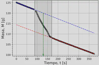
In this figure you can see 3 regions, the leftmost one where the mass is decreasing at a steady rate (the liquid nitrogen evaporating at the surface), the shaded region where the mas decreases at a faster rate than before due to the sample entering the liquid and exchanging heat with it, and the rightmost region where the sample and the nitrogen have reached thermal equilibrium and the mass decreases at the same rate as initially.
We are interested in measuring the change of mass in the shaded region. To do this, we do a linear fit of the data in the first and third regions, extrapolate these lines, and find the difference between the two at the midpoint of the shaded region. This way we know $\Delta M$.
Having done this, we can then find the heat capacity value for the used sample. As you can probably tell, this was a tiresome process since we had to do the manual analysis of the videos for a set of different samples. It’s because of this that we later decided to automate this experiment as part of the course ‘Digital Electronics’.
Automating the experiment
There’s many parts of the experiment that can be automated. In our approach we automated:
- The measuring of the sample’s mass
- Placing the sample inside the container
- Taking the sample out of the container
- Measuring the mass over time
- Plotting the intended figure
- Calculating the heat capacity
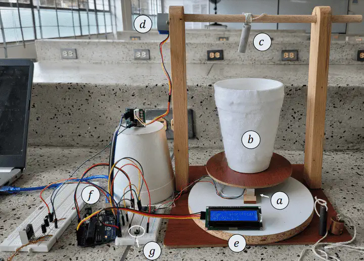
We did this using the experimental setup that is shown next:
All of these elements were handled by the arduino board while a python script was doing the real-time plotting as well as the analysis once the experiment concluded. The developed codes can be found here.
Briefly said, the automated experiment is carried out like this: First, the user is prompted by a console message to provide the element’s symbol of the sample, then the LCD screen tells the user to place the sample (already tied to the rotating stick) on top of the scale to measure its mass. After this, the user is asked to press the button to lift the sample up. Once the sample is up, the LCD tells the user to place the liquid nitrogen on the scale. Once the system detects the nitrogen is on the scale, it displays its mass, and prompts the user to press the button to start the experiment. The program then starts to store the mass values and display them in a real-time plot for the user to see, while also showing the current mass and time in the LCD. After 20 seconds, the sample starts to come down, entering the liquid nitrogen shortly after. The program then uses the data to detect when thermal equilibrium has been reached, and 20 seconds after that it stops the experiment, shows the final plot, and lifts the sample up. The user is asked to remove the nitrogen from the scale, the sample is brought down, and the heat capacity is shown in the LCD.
A video of the automated experiment being carried out can be seen next:
Having done the experiment both manually and in an automated manner, we saw that the relative errors of the found values of heat capacity of different materials were smaller when using the automated setup. With this, automating the experiment not only made it faster to analyse and reduced the manual work performed by the user, but it also allowed the user to obtain more accurate results.
Resources
Acknowledgments
This project was done by me and Lizeth González